In everyday maths, a proportion is an equation that says two ratios are equal, like 3/4 = 9/12. In statistics the word means something slightly different, and the difference trips up a lot of students. Here, a proportion is the share of a group that has some feature: the fraction of voters who back a candidate, of light bulbs that fail early, of website visitors who buy something.
This guide covers what a statistical proportion is, how it differs from a mathematical one, and how the core tools of inference (standard error, confidence intervals, hypothesis tests and sample size) are built on it. Each section links to a free calculator that does the arithmetic with every step shown.
Population Proportion vs Sample Proportion
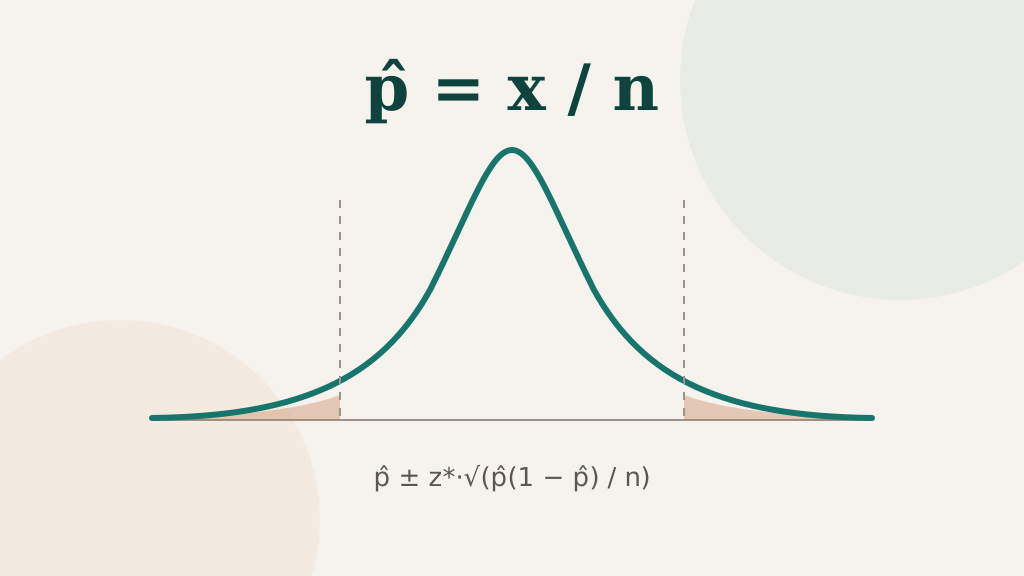
A population proportion p is the true share of a whole population with some feature, while a sample proportion p̂ = x ÷ n is the share observed in a sample and used to estimate p. The population value is fixed but usually unknown; the sample value changes from one sample to the next.
There are always two proportions in play.
- The population proportion, p. The true share of the whole population with the feature. It’s a fixed number, but you almost never know it, because you can’t survey everyone.
- The sample proportion, p̂ (“p-hat”). The share in the sample you actually collected: p̂ = x ÷ n, where x is the number of “successes” and n is the sample size.
If 168 of 400 surveyed households own a dog, then p̂ = 168 ÷ 400 = 0.42. That 0.42 is your best estimate of p, but a different random 400 households would give a slightly different p̂. The rest of statistics for proportions is about handling that variation honestly. The sample proportion calculator computes p̂ and everything that follows from it.
How this connects to ratios
A sample proportion is a part-to-whole ratio, x : n, written as a decimal. Converting 168 : 400 to 0.42 is exactly what the ratio to decimal calculator does, and stating it as “42%” is a percent proportion. What statistics adds is the question: how much would this ratio change if I drew a different sample?
What Is the Standard Error of a Proportion?
The standard error of a proportion measures how much p̂ typically varies from sample to sample. For 168 dog-owning households out of 400, p̂ = 0.42 and the standard error is about 0.0247, and it shrinks as the sample grows.
The spread of p̂ from sample to sample is measured by its standard error:
SE = √( p̂ (1 − p̂) ÷ n )
For the dog survey, SE = √(0.42 × 0.58 ÷ 400) ≈ 0.0247, about 2.5 percentage points. Two features of this formula drive almost every practical decision:
- It shrinks with √n, not n. Quadrupling the sample only halves the standard error.
- It is largest at p̂ = 0.5. Proportions near 50% are the hardest to pin down; proportions near 0 or 1 are easier.
When np ≥ 10 and n(1 − p) ≥ 10, the distribution of p̂ across samples is approximately normal, centred on p. That’s why z-scores and the normal curve appear in every method below.
Confidence Intervals for a Proportion
A confidence interval for a proportion is a range of plausible values for p, built as p̂ plus or minus a margin of error. For p̂ = 0.42 from 400 households, the 95% interval is about 0.42 ± 0.048, or roughly 37.2% to 46.8%.
A confidence interval turns p̂ and its standard error into a range of plausible values for p:
p̂ ± z × SE*
At 95% confidence, z* = 1.96. In a poll where 540 of 1,200 people support a proposal, p̂ = 0.45, SE ≈ 0.0144, and the margin of error is 1.96 × 0.0144 ≈ 0.028. So the interval is 42.2% to 47.8%. This is the “±3 points” you see quoted with opinion polls.
That textbook formula (the Wald interval) breaks down for small samples or proportions near 0 or 1. It can even produce a negative lower bound. The Wilson score interval fixes this and is the modern default. The confidence interval for a proportion calculator shows Wald, Wilson and Agresti–Coull side by side, so you can see when they agree and when they don’t.
To estimate the difference between two groups, such as support among under-30s versus over-60s, use the two proportion confidence interval calculator, which builds an interval for p₁ − p₂.
Hypothesis Tests for Proportions
A hypothesis test for a proportion checks whether the data are consistent with a claimed value. The one-proportion z-test compares one sample with a claimed p₀, and the two-proportion z-test compares two independent groups; both turn the gap into a z statistic and a p-value.
One proportion: testing a claim
Is a coin that lands heads 62 times in 100 tosses fair? The one-proportion z-test compares p̂ with a claimed value p₀:
z = (p̂ − p₀) ÷ √( p₀ (1 − p₀) ÷ n )
Here z = (0.62 − 0.5) ÷ 0.05 = 2.40, and the two-tailed p-value is 0.0164. Below 0.05, so we reject the claim that the coin is fair. Note that the standard error uses p₀, not p̂, because the test asks what would happen if the claim were true. Run your own with the one proportion z-test calculator.
Two proportions: comparing groups
Did version B of a web page convert better than version A? The two-proportion z-test pools both samples under the null hypothesis that they share one proportion:
z = (p̂₁ − p̂₂) ÷ √( p̂ (1 − p̂)(1/n₁ + 1/n₂) )
With 120/1,000 conversions for A and 150/1,000 for B, the pooled proportion is 0.135, z ≈ −1.96 and p ≈ 0.0496. That’s significant at 5%, but only just. The two proportion z-test calculator also reports the relative lift (25% here) and checks the sample-size conditions.
How Many People Do You Need? Sample Size for a Proportion
The sample size needed to estimate a proportion is n = z*² · p(1 − p) ÷ E². At 95% confidence with no prior estimate (p = 0.5), a margin of ±3 points needs 1,068 people and ±5 points needs 385.
Rearranging the margin-of-error formula gives the sample size needed for a target precision:
n = z*² × p(1 − p) ÷ E²
With no prior estimate, use p = 0.5, the most conservative choice. For ±3 points at 95% confidence: n = 1.96² × 0.25 ÷ 0.03² ≈ 1,067.1, which rounds up to 1,068. That’s why so many national polls survey about a thousand people. When you’re sampling a large share of a small population, a finite population correction reduces the number. The sample size for a proportion calculator handles both.
| Margin of error (95%, p = 0.5) | Sample size needed |
|---|---|
| ±10% | 97 |
| ±5% | 385 |
| ±3% | 1,068 |
| ±2% | 2,401 |
| ±1% | 9,604 |
What Conditions Do Proportion Tests Need?
Proportion tests and intervals based on the normal distribution need a random sample, independent observations, and at least 10 expected successes and 10 expected failures.
All of these normal-based methods share the same assumptions:
- Random sample (or random assignment, in an experiment).
- Independence. When sampling without replacement, the sample should be under about 10% of the population.
- Large enough counts. At least 10 expected successes and 10 expected failures.
If the counts are small, prefer exact methods: the Wilson interval for estimation, and an exact binomial or Fisher’s test for hypotheses.
Math Proportion vs Statistical Proportion
A math proportion is an equation between two ratios, solved by cross multiplication; a statistical proportion is a single part-to-whole ratio used to estimate a population share. To solve a math proportion such as 3/4 = x/12, use the proportion calculator. The table compares the two meanings.
| In maths | In statistics | |
|---|---|---|
| What it is | An equation: two ratios are equal (a/b = c/d) | A share of a group with a feature (x / n) |
| Typical question | Find the missing term | Estimate p, or test a claim about it |
| Key tool | Cross multiplication | Standard error and the normal curve |
| Example | 3/4 = x/12 → x = 9 | 540 of 1,200 → 45% ± 2.8% |
Both ideas rest on the same object, a ratio of part to whole. If you’re new to the maths side, start with what a proportion is and the difference between a ratio and a proportion. For the statistical side, the proportion statistics calculators cover the full workflow, from planning a sample to reporting a test.